Research Problems in Pretraining

Pretraining is a single optimization problem. Minimize next-token prediction loss. Cross-entropy, backpropagation, some gradient-based optimizer. That is the entire algorithm. The rest is scale, and scale changes everything.

This post is a practitioner’s map of the pretraining research landscape, adapted from a talk I gave at the Stanford Math Department Student Learning Symposium. It is not a survey. It is closer to what the terrain looks like from inside the cockpit: where the clean theory is, where it breaks down, and where the open questions sit.

The optimization problem

At its core, pretraining trains a model to predict the conditional distribution $P(x_{t+1} \mid x_1, \ldots, x_t)$ over a vocabulary, given a prefix of tokens. The loss is cross-entropy between the model’s predicted distribution and the ground truth. Training uses teacher forcing: at each step, the model conditions on the actual previous tokens from the training data, not its own predictions.

This formulation has not changed since the early language modeling days. What changed is the scale: trillions of parameters, tens of trillions of tokens, months of GPU time.

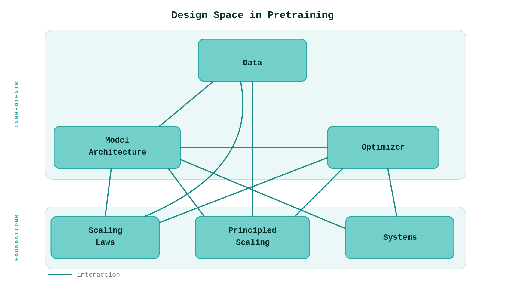
The design space

Pretraining sits at the intersection of six areas, each a research field in its own right:

1. Scaling laws — given a compute budget, how should you allocate between model size and data?
2. Model architecture — dense vs. Mixture-of-Experts, attention variants, KV sharing, hybrid local/global patterns.
3. Data selection and mixture — which data, in what proportions, in what order?
4. Optimizers — learning rate, batch size, scheduler, and the choice of optimizer itself.
5. Principled scaling / parameterization — how to transfer hyperparameters from small proxy models to the target scale.
6. Systems — parallelism strategies (tensor, pipeline, data, expert), MFU optimization, co-design constraints.

The search space is high-dimensional. Each axis interacts with every other. Architecture choices constrain system efficiency. Data mixture changes the optimal learning rate. Batch size depends on both optimization dynamics and hardware utilization. Joint optimization across all six is intractable, so practitioners decompose: hold five fixed, sweep one, hope the interactions are weak enough. Sometimes they are. Sometimes they are not.

Data quality deserves its own callout. Low-quality data does not merely add noise; it actively degrades knowledge retention from good data by roughly an order of magnitude in efficiency terms (a figure from practitioner experience rather than a single published study). Modern data pipelines are sophisticated but remain largely intuition-driven, with domain-specific filtering heuristics layered on top of general deduplication. DoReMi reframes mixture selection as minimax optimization, and RegMix treats it as regression. Both are steps toward principled data curation, but the field is far from solved.

The cost of being wrong

To make the stakes concrete, consider a rough calculation for a frontier model.

A Mixture-of-Experts model with roughly 100B active parameters (out of perhaps 10T total) trained on 100T tokens requires approximately $6 \times 10^{25}$ FLOPs (this standard $6ND$ approximation excludes activation recomputation overhead from gradient checkpointing, which adds roughly 33%). One H100-hour delivers about $3.6 \times 10^{18}$ FLOPs. Training efficiency, measured as Model FLOPs Utilization (MFU, the fraction of theoretical peak FLOPs actually spent on useful computation), ranges from 20% to 35% for frontier runs, depending on the parallelism strategy and communication overhead. That puts the H100-hour requirement between $4.9 \times 10^7$ and $8.3 \times 10^7$. At contract prices of $2.00—2.70 per H100-hour, the total cost lands between $98M and $225M.

Every design decision — architecture, data mixture, learning rate schedule, optimizer — is a bet you are placing with that budget. You cannot afford to grid-search at the target scale. You need a way to run cheap experiments at small scale and predict what happens at large scale. That is what scaling laws are for.

Scaling laws: the empirical backbone

Scaling laws are the empirical observation that test loss follows a power-law relationship with model size, data size, and compute. The foundational formulations come from Kaplan et al. (2020), who established the power-law structure, and Hoffmann et al. (2022), who derived the compute-optimal allocation (the “Chinchilla” result).

The Chinchilla form is:

$L(N, D) = E + \frac{A}{N^\alpha} + \frac{B}{D^\beta}$

where $N$ is model size, $D$ is data size, $E$ is the irreducible entropy of the data source, and $\alpha$, $\beta$ are fitted exponents. The second term is the penalty for insufficient parameters; the third, the penalty for insufficient data. Both penalties shrink as power laws, which is why scaling works at all. Optimizing this subject to a compute constraint $C \propto N \cdot D$ yields the familiar result that both $N$ and $D$ should scale roughly as $C^{0.5}$. This was a significant correction to Kaplan et al., who had recommended scaling model size much faster ($N \sim C^{0.73}$) while underinvesting in data. The Chinchilla result showed that balanced allocation, scaling both model and data equally, is substantially more compute-efficient.

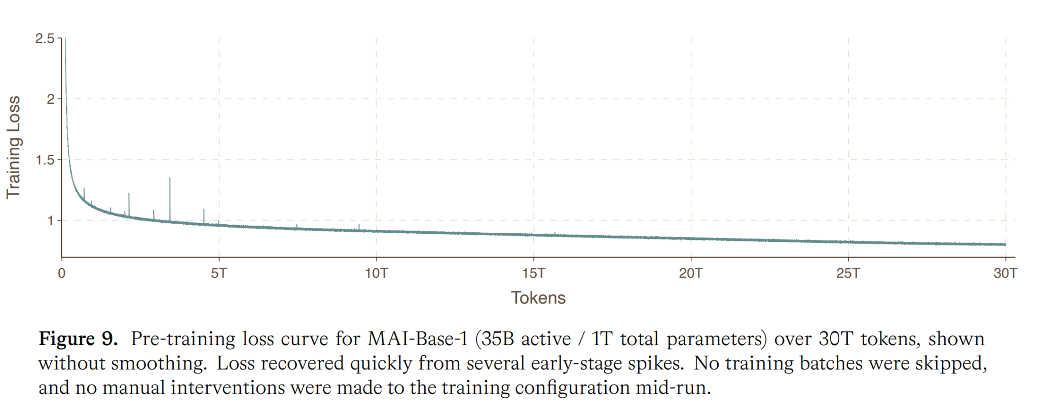From MAI-Thinking-1 technical report, Microsoft.

I have written separately about the math behind compute-optimal training in detail, including the derivation and its practical implications. Here I want to focus on how scaling laws are used in practice and where they break.

The MoE setting introduces additional dimensions: sparsity, granularity, expert count, and active parameters. Clark et al. (2022) extended scaling laws to routed models, and Krajewski et al. (2024) refined the functional forms further. Muennighoff et al. (2023) addressed the data-constrained regime, where tokens must be repeated.

The scaling ladder workflow

The practitioner’s workflow looks like this:

1. Train a “ladder” of small models at increasing compute budgets.
2. Fit the scaling law parameters to the observed losses.
3. Extrapolate to the target compute budget.
4. Use the extrapolation to set model size, data size, and other hyperparameters.

This is powerful. Scaling laws enable roughly 300x extrapolation, meaning you can predict the loss of a model that would cost $100M to train from experiments costing a few hundred thousand dollars. The ladder converts each design decision from a $M gamble into a $K experiment.

Two concrete techniques within this workflow:

Isoflop sweeps. Fix a compute budget. Train models of various sizes (adjusting token count to keep FLOPs constant). Plot loss vs. model size. The minimum gives you the loss-optimal model size for that compute level. Repeat at several compute budgets, and you trace out the compute-optimal frontier.

Treatment comparison. Fit parallel $L(C)$ curves for design variant A and design variant B. Extrapolate both to the target scale. The gap at the target is your estimated effect size. This lets you compare architectures, data mixtures, or optimizer configurations cheaply.

Where it gets hard

Signal-to-noise is the first problem. Small models are noisy. Individual benchmark results at the 1B-parameter scale carry limited information about 100B-scale behavior. Practitioners cluster benchmarks, use soft evaluation metrics, and average aggressively. Even so, some effects only appear at scale.

There is a deeper structural problem: the scaling laws for compute-optimality and for architecture optimization may use incompatible functional forms. Compute-optimal scaling relates loss to $(N, D)$. Architecture comparisons often need richer parameterizations. Joint optimization across both remains open.

Predicting post-training performance from pre-training loss is unreliable for specific capabilities. A model with lower pre-training loss generally performs better after instruction tuning and RLHF, but the correlation is noisy for narrow tasks. One practical trick: stochastic weight averaging of checkpoints along the training trajectory approximates post-cooldown performance, enabling cheaper early decisions without running the full learning rate decay (Hagele et al. 2024).

Finally, MFU-aware comparison matters. Two training configurations may achieve the same loss-per-FLOP but different loss-per-GPU-hour, because one has better hardware utilization. Comparing in (GPU-hours, accuracy) space rather than (FLOPs, loss) space gives you the economically relevant answer.

Principled scaling: from small to large

Scaling laws tell you what to expect at target scale. Principled parameterization tells you how to get there without re-tuning hyperparameters.

The core problem: standard parameterization (SP) causes feature learning dynamics to change with model width. At small width, the model learns features. At large width, under SP, the updates either vanish or explode relative to the activation scale. The model that worked at 1B parameters does not train with the same hyperparameters at 100B.

muP: Maximal Update Parameterization

Yang et al. (2022) solved this with muP (Maximal Update Parameterization, from the Tensor Programs series). The key idea: scale initialization variances, learning rates, and output multipliers so that the “maximal update” at each layer remains $\Theta(1)$ regardless of width.

Under muP, the optimal learning rate transfers across scales. You tune at a small proxy width, then deploy at the target width with the same learning rate. This is not a minor convenience; it eliminates one of the most expensive hyperparameter searches in pretraining.

From Microsoft Research blog on muTransfer.

Everett et al. (2024) systematically compared SP, muP, and intermediate parameterizations by characterizing scaling exponents for initialization and learning rate as a function of width. Their key finding complicates the muP narrative in a productive way: hyperparameter transfer is not unique to muP. Under the right choice of scaling exponents, all parameterizations can achieve transfer. muP is the specific choice where feature learning is width-independent, but it is not the only path to scale-invariant training dynamics.

Work on SP-full-align (sometimes called Complete P) extends muP to handle all layers uniformly, including embeddings and the final projection, addressing edge cases where the original muP prescription left some layers in the SP regime.

Critical batch size

McCandlish et al. (2018) introduced the critical batch size $B_{\text{crit}}$, defined roughly as the batch size where gradient noise matches the gradient signal. Below $B_{\text{crit}}$, doubling the batch size gives near-linear speedup (each gradient is informative). Above $B_{\text{crit}}$, you get diminishing returns (the gradient is already accurate enough, and extra samples are redundant).

This creates a direct link between optimization theory and systems engineering. The “right” batch size is not purely an optimization question or purely a hardware utilization question. It is both.

The optimizer frontier

Principled parameterization tells you how to set hyperparameters so they transfer across scales. But which optimizer those hyperparameters belong to is itself a design choice, and the frontier here has shifted significantly in the past two years.

AdamW: the baseline

AdamW has been the dominant optimizer for LLM pretraining since GPT-2. Per-parameter adaptive step sizes via first and second moment estimates, with decoupled weight decay. It works. It is well understood. Nearly all scaling law results are calibrated against it.

Muon: spectral optimization

Muon (Jordan et al., 2024) takes a different approach, grounded in the theory of modular duality developed by Bernstein and Newhouse (2024). It orthogonalizes gradient updates via Newton-Schulz iteration (an iterative method for computing the polar decomposition of a matrix), replacing each update with its nearest semi-orthogonal matrix so that the update has unit spectral norm. The weight matrices themselves are not constrained to be orthogonal.

Orthogonalizing the update addresses a specific problem in transformer hidden layers: raw gradient updates tend to be dominated by a few singular directions, so most of the update’s energy concentrates along those directions while others are starved. By equalizing the singular values of the update, Muon distributes learning across all directions, enabling a higher critical batch size (you can use larger batches before hitting diminishing returns). The relationship to prior work is precise: Muon is an accumulation-free variant of Shampoo, computing the spectral preconditioning instantaneously from each step’s gradient rather than maintaining running statistics.

Scion: the unifying view

Pethick et al. (2025) provide a unifying framework via Frank-Wolfe optimization (a projection-free method that optimizes over a constraint set by solving linear subproblems) over norm balls. The key insight: the choice of norm ball determines the optimizer’s behavior. The spectral norm ball recovers Muon. The $\ell_\infty$ ball gives you SignSGD. The $\ell_2$ ball gives you normalized gradient descent.

This is clarifying. Instead of treating each optimizer as a separate invention, Scion reveals them as instances of a single principle: constrain the update to a norm ball, and the geometry of that ball dictates the optimization dynamics. The spectral norm ball interpretation also connects Muon and SOAP through the shared structure of their preconditioners.

Learning rate scheduling

Cosine decay has been the default schedule, but it requires committing to a total training duration upfront. WSD (Warmup-Stable-Decay) offers a practical alternative: a warmup phase, a stable phase at peak learning rate, and a short decay phase. The key advantage is that you can checkpoint during the stable phase and branch off decay runs at any point, enabling cheaper continuation experiments and anytime evaluation.

The open mysteries

The clean power-law structure of scaling laws is empirically robust. But nobody has derived it from first principles. Several partial theories offer different angles:

The quantization hypothesis. Michaud et al. (2024) propose that the network learns discrete “quanta” of skill. Each quantum has a difficulty threshold. The power law emerges from the distribution of difficulties across quanta. This is appealingly concrete but hard to test directly.

Learning curve theory. Hutter (2021) gives an information-theoretic argument for why learning curves should follow power laws, connecting to compressibility of the data source.

Dynamical mean field theory. Bordelon, Atanasov, and Pehlevan (2024) derive scaling behavior from infinite-width dynamics, grounding the empirical laws in statistical physics.

Generalization dynamics. Recent work explores mode-hopping and phase transitions during training as mechanisms that produce the observed scaling structure. The loss does not decrease smoothly; it stalls, then drops, then stalls again. These transitions may be related to the network discovering qualitatively new representations.

Simon et al. (2026) argue that power laws are one pillar of an emerging “learning mechanics,” a theoretical framework that would unify scaling, generalization, and optimization dynamics.

Beyond scaling laws, several questions sit at the frontier:

• Emergent properties. Some capabilities appear abruptly at scale, both positive (in-context learning, chain-of-thought reasoning) and negative (new failure modes). Predicting which capabilities emerge and when remains unreliable.
• Hyperparameter transfer mechanisms. muP works empirically, but the deeper question of why certain parameterizations enable transfer while others do not connects to open problems in high-dimensional optimization theory.
• Optimal architecture for compression. Given a fixed compute budget, what architecture maximizes the information extracted from the training data? The MoE setting adds a twist: router normalization may accidentally impose manifold constraints on optimization that happen to be beneficial.

Closing

Pretraining research is in an unusual position. The empirical regularities are strong enough to guide billion-dollar decisions. The theoretical foundations are thin enough that practitioners regularly encounter phenomena they cannot explain. The field advances by interleaving careful empiricism (scaling ladders, isoflop sweeps, treatment comparisons) with theoretical conjectures (muP, spectral optimization, quantization hypotheses) and engineering discipline (MFU optimization, stability monitoring, systems co-design).

The open questions are not peripheral curiosities. Why power laws exist determines whether the current scaling paradigm has a ceiling. How hyperparameter transfer works determines whether proxy experiments remain reliable at the next order of magnitude. What causes phase transitions during training determines whether we can predict emergent capabilities before they appear.

For mathematicians looking at this field: the problems are real, the data is abundant, and the gap between theory and practice is wide enough to drive meaningful contributions through.